Modular Production Line Optimization:
The ExPLOre Architecture1
| Diomidis D. Spinellis | Chrissoleon T. Papadopoulos |
| |
| Department of Information and Communication Systems | Department of Business Administration |
| GR-832 00 Karlovasi | GR-821 00 Chios |
| University of the Aegean | University of the Aegean |
| Greece | Greece |
| dspin@aegean.gr | hpap@aegean.gr |
Abstract
The general design problem in serial production lines concerns
the allocation of resources such as the number of servers, their service
rates, and buffers given production-specific constraints,
associated costs, and revenue projections.
We describe the design of exPLOre:
a modular, object-oriented,
production line optimization
software architecture.
An abstract optimization module
can be instantiated using a variety of stochastic optimization methods
such as simulated annealing and genetic algorithms.
Its search space is constrained by a
constraint checker while
its search direction is guided by a
cost analyser which combines the output of a
throughput evaluator with the business model.
The throughput evaluator can be instantiated using
Markovian, generalised queueing network methods,
a decomposition, or an expansion method algorithm.
Keywords:
Manufacturing systems;
production lines;
stochastic modeling, analysis;
performance evaluation, optimization.
AMS Classification: 90C15 Stochastic programming
1 Introduction
Serial production lines form the heart of many manufacturing systems.
Their optimal design is subject to specific constraints, associated
costs, and revenue projections.
Much of the research in this field concerns the design of these
manufacturing systems when there is considerable inherent
variability in the processing times at the various stations,
a common situation with human operators/assemblers.
The general design problem in serial production lines involves
the allocation of resources such as the number of servers, their service
rates, and buffers at each of the servers.
These problems are called,
respectively, the server allocation, the workload allocation, and the
buffer allocation problems.
The problem mentioned above is a nonlinear stochastic problem. One of
its features which makes it very challenging to solve is that no known
closed-form expression for estimating the throughputs of the lines
exists. This characteristic makes it very difficult to control the design
variables as a function of the variation in the objective function.
For a systematic classification of the relevant
works on the stochastic modeling of these and other types of
manufacturing systems (e.g., transfer lines, flexible
manufacturing systems (FMS) and flexible assembly systems (FAS)),
the interested reader is referred to a review paper
by Papadopoulos and Heavey [1] and
some recently published books, such as Askin and
Standridge [2],
Buzacott and Shanthikumar [3], Gershwin [4],
Papadopoulos et al. [5],
Viswanadham and Narahari [6], and Altiok [7].
The difficulties of the problem have led us towards the deployment
of an arsenal of different methods for determining the optimal
design of the production line.
These methods involve both the estimation of line throughput and
the calculation of the optimal line design variables.
In this paper we describe the design of exPLOre:
a modular, object-oriented,
production line optimization software architecture.
Up to now we have used the system
for solving the buffer allocation problem in production lines with
well over 100 stations in series [8],
and for investigating the allocation buffers, servers, and service rates in
production lines with up to 60 stations in series.
The rest of this paper is organised as follows:
in section 2 we present the mathematical model of
the production line,
in section 3 we describe the exPLOre architecture,
in section 4 we present the exPLOre prototype
implementation and some initial results,
while section 5 concludes the paper with a description
of our future plans.
2 The Production Line Model
The production line decision model we used is based on the optimal
allocation of its constituent resources namely:
the number of servers,
their service rates,
and buffers at each of the servers.
The effect of the number of servers and the service rates on the production
throughput and cost is obvious: an increased number of servers or service
rate can be readily associated with a given cost and will increase the
line throughput by a specific measure.
The effect of the production line buffer allocation in terms of
throughput and cost is more subtle.
The main purpose of buffers in production or flow lines is to give each
stage of a system some degree of independence from the rest of the
system. If buffers were non-existent then the only way two connected
workcenters could operate would be in perfect synchronization;
a utopian situation. If there were no buffers between two workcenters
at least one of two situations would occur:
``blocking'' of the first station or ``starving'' of the second station.
Blocking of the first station occurs when the first station finishes
processing its stock and releases it before the second station completes
the material it is working on and the buffer of the second station is
full. Starving occurs when the second station completes its work yet
there are no parts in its buffer because the first workcenter is either
busy or has no work.
In both cases the system throughput is below the expected.
One other situation that leads to loss of capacity is
the breakdown of a workcenter in the line.
If there are no buffers, all the stations of the system have
to shut down either because of starving or blocking. If there are
buffers between the stations the remaining stations can keep operating
for some time. In allocating buffers the number of buffers is not only
dependent upon the processing parameters of the production line but
also upon the positions of stations within the line. Another feature of
buffers is that buffers cease to be effective after some quantity.
Beyond a threshold quantity of buffers the increase in the overall
output of the line is overridden by the costs associated with buffers.
Although buffers are an essential part of any production line with
finite capacities, there are costs associated with buffers. One of the
important costs of buffers is the effect on flow time. Flow time is the
time required to move a piece through the system process from entry to
completion of the last stage. Customers accumulate indirect costs
proportional to the time spent in the system. An increase results in
high flow time to processing time ratios and thus reduced output.
Another area of cost is the cost due to occupation of space. Larger
quantities of buffers mean more space is occupied for waiting which
otherwise could be used for processing equipment or faster movement of
material handling equipment. Handling the unit into and out of the
in-process inventory banks also adds to the costs.
From this description one can see that determining the quantity of
buffers for each station in order to create perfect balance between the
costs and benefits associated with buffers is a challenging task.
Based on a given setting of the resources described above we can calculate
two objective measures of the line's operation:
the average throughput and the average work in progress i.e.
the average total number of units in the production line at
steady state.
Taking into account the average revenue per item, its associated
variable production cost and holding cost, and the costs of deploying
the resources we described above we can obtain an objective measure
of the line's economic performance.
Thus the production line under investigation can be modeled
using the following basic objective function:
|
|
max
| Z = X (R-V) - h L - CB |
K
�
i = 2
|
qi - |
K
�
i = 1
|
CSisi - |
K
�
i = 1
|
CRi |
| (1) |
where
- K is the number of individual stations within the line,
- X is the average throughput of the line,
- R is the average revenue per item,
- V is the average variable production cost,
- h is the average holding cost per item,
- L is the average WIP,
- CB is the cost of providing one unit of buffer space,
- qi is the buffer capacity allocated at buffer location i,
- CSi is the cost of a server at location i,
- si is the number of servers per workstation i, and
- CRi is the cost of obtaining a given service rate at workstation
location i.
3 The exPLOre Architecture
The exPLOre architecture is used for building customized, flexible,
and efficient production line optimization decision support systems.
The modularity of the system allows
the utilization of different evaluative function and optimization methods
as well as
the parametric expression of the production line constraints and the business
model.
This flexibility is needed so that the system's user can choose the
appropriate algorithms for solving the problem at hand.
The guiding tradeoffs between the different modules concern their
relative efficiency, accuracy, and applicability.
As an example it is possible to obtain an exact buffer configuration
for a small production line using full enumeration and the decomposition
method.
On the other hand, in order to obtain a buffer and server number allocation
for a large production line one would choose simulated annealing as the
optimization method because the full enumeration of all configurations
would take a prohibitive long time to complete, and the expansion method
as the evaluative function because the decomposition method
we utilize in our current implementation does not deal with parallel servers.

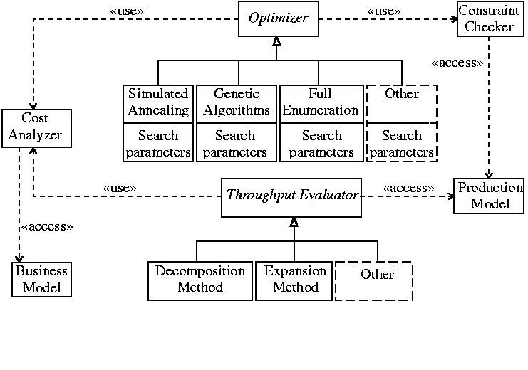
Figure 1:
The exPLOre architectural model.
The exPLOre architecture is graphically depicted,
as a UML class diagram [9], in Figure 1.
The architecture's driver is an abstract optimization module.
This can be instantiated using a variety of optimization methods such as
simulated annealing,
genetic algorithms, or even the exhaustive (or reduced)
enumeration of the search space.
The search space of the optimizer is constrained by the output of the
constraint checker which,
based on a production model expressed in
a declarative domain-specific language [10],
acts as an ``oracle'' determining the allowed line configurations.
The search direction of the optimizer is guided by the
cost analyser which combines the output of the
throughput evaluator with variables from the business model
to determine the objective merit of a given line configuration.
The business model specifies the business benefit of a given
line throughput as well as the business costs associated with the
resources that are used to obtain that level of throughput.
The abstract throughput evaluator can be instantiated using
Markovian, generalised queueing network methods,
a decomposition, or an expansion method algorithm.
4 Prototype Implementation
In order to test the viability of the exPLOre architecture we have
implemented a number of concrete modules for the optimizer and
the throughput evaluator.
Based on those modules we were able to obtain optimal production
line configurations for both small and large production lines
within acceptable execution time constraints (e.g. Figure 3).
In the following paragraphs we outline the modules that we have implemented.
4.1 Full Enumeration Optimizer
The full enumeration optimizer
determines the optimal line configuration by an exhaustive enumeration
of all possible configurations.
It is viable only for small production lines, servers, and buffer space.
However, it is
useful for cross-checking the results of other optimization methods.
All buffer (and server) combinations can be methodically enumerated by
considering a vector p denoting the position within
the production line of each one of the Q available buffers.
If we use
q = (q2,q3,�,qK)
then
given the vector p we can then easily map
p to q
using the following equation:
For example
p = (1, 2, 2, 2, 4, 1)�q = (2, 3, 0, 1).
If we then define a recursive function g as
|
g(p, l) = |
�
�
�
�
�
�
�
�
�
�
�
|
|
| |
|
|
|
( |
p�l+1, �, p�l+1
l
|
, p�l+1, p�l+2, �) |
|
|
|
|
| |
|
|
| (3) |
given an initial buffer configuration of Q buffers
we can sequentially advance
through each next possible configuration p� by setting
Essentially, g maps the vector of positions to a new one
representing another line configuration.
When the incremented position pi of a buffer resource i
reaches K, the last place in the line, (pi + 1 = K)
then
g is recursively applied setting l to point to the buffer
in position pi+1.
The result of the recursive application of g is then adjusted by
setting the values from p1 to pl to the new value of
p�i+1.
The complete enumeration terminates when all buffers reach
the line position K.
As an example, in a line consisting of 3 buffers and 2 stations
(Q = 3, K = 2) p and q will take
the following values:
The above procedure is also used for obtaining all different server
combinations.
To enumerate all buffer and server combinations one complete
server enumeration is performed for each line buffer configuration.
4.2 Reduced Enumeration Optimizer
A variant of the full enumeration optimizer uses a
reduced enumeration procedure
by skipping non-viable buffer allocation configurations.
Reduced enumeration is based on the experimental observation that the absolute
difference of the respective elements of the optimal buffer allocation (OBA)
vectors with N and N+1 buffer slots is less than or equal to 1:
|
|qiN+1 - qiN| � 1, "i: 2 � i � K. |
| (7) |
i.e. once the OBA for a given value N of the number of the
total buffer slots that have to be allocated among the intermediate buffers
of the production line has been determined,
the OBA for a value N+1 can be found by allocating the extra buffer slot
in one of the neighbouring buffer locations of the previous optimal buffer
allocation.
In this way, we have been able to derive the OBA by induction for any number
N of buffer slots that are to be allocated among the K-1 buffer locations
of the line.
The reduction works as follows: when N* and K are given one
needs to determine all the OBA vectors for N = 1,2,�,N* and then for
N = N*+1 by searching only the values of qiN-1, qiN and
qiN+1.
Furthermore, this reduction starts after a number of total
buffer slots N.
The reduction is substantial: by applying the improved
enumeration it has been experimentally observed that the number of iterations
were reduced by at least 60% for short lines.
This reduction accounts for well
over 90% for large production lines (with more than 12 stations).
4.3 Simulated Annealing Optimizer
The simulated annealing (SA) optimizer
determines a near-optimal configuration using the SA
[11,12] stochastic algorithm.
Its search parameters may need expert problem-specific tuning.
Simulated annealing is an adaptation of the simulation of physical
thermodynamic annealing principles described by
Metropolis et al. [13]
to the combinatorial optimization problems [14,11].
Similar to genetic algorithms [15,16] and
tabu search techniques
[17] it follows the ``local improvement'' paradigm for
harnessing the exponential complexity of the solution space.
The algorithm is based on randomization techniques.
An overview of algorithms based on such techniques can be
found in the survey by Gupta et al. [18].
A complete presentation of the method and its applications
is described by Van Laarhoven and Aarts [12]
and accessible algorithms for its implementation
are presented by Corana et al. [19]
and Press et al. [20].
As a tool for operational research SA is presented
by Eglese [21],
while Koulamas et al. [22] provide a complete survey of
SA applications to operations research problems.
In our implementation [8],
we found that the algorithm
can handle large configurations in bounded execution time.
4.4 Genetic Algorithm Optimizer
The genetic algorithm (GA) optimizer
determines a near-optimal configuration using genetic algorithms.
Genetic algorithms [15,16,23,24]
are global optimization techniques that
avoid many of the shortcomings exhibited by local search techniques on
difficult search spaces, such as the buffer allocation problem.
Genetic algorithm applications are outlined by Goldberg [25],
their use for modeling, design, and process control is presented by
Karr [24],
while the methodology used for optimizing simulated systems can be found in
the work by Tompkins and Azadivar [26].
GAs rely on modeling the problem as a population of organisms.
Every organism represents a possible valid solution to the problem.
Organisms are composed of alleles representing parts of
a given solution.
Standard genetic recombination operators are used to
create new organisms out of existing ones by combining
alleles of the existing organisms.
In addition, mutations can randomly change the composition of
existing organisms.
Typically, the algorithm
evaluates all the organisms of the population and creates
new organisms by combining existing ones based on their
fitness.
This procedure is repeated until the variance of the population reaches
a predefined minimum value.
The GA optimizer can also handle large configurations in bounded execution
time.
We found [27] that
the optimizer typically executes faster than the simulated annealing optimizer,
producing however less optimal configurations.
4.5 Exact Evaluator
The exact evaluator uses an exact numerical algorithm [28]
in conjunction with a traditional Markovian state model.
It provides an exact measure of the line throughput at the expense
of prohibitively large execution times.
Our implementation only handles lines with variable buffer allocations.
The evaluator is
mostly useful for small lines with a limited number of buffers, or
for verifying the operation of the other evaluators.
4.6 Decomposition Method Evaluator
The decomposition method evaluator is a
throughput evaluator based on the decomposition method [29,30].
Compared with the exact evaluator it
provides an efficient and relatively accurate approximation of the line
throughput.
Our implementation
can not handle parallel servers and variable service rates.
4.7 Expansion Method Evaluator
The Expansion Method is a robust and effective approximation technique
developed by Kerbache and Smith [31].
This method is characterized as a
combination of Repeated Trials and Node-by-node Decomposition solution
procedures.
In contrast to our decomposition method evaluator, the expansion
method evaluator
can handle arbitrary line topologies with parallel server and variable
service rates.
Its evaluative efficiency is however worse than the decomposition method
evaluator.
4.8 Application Scenarios
Based on the above modules we obtained near-optimal line configurations
for a number of different buffer, server, and service rate allocation
problems for both large and small production lines.
As a representative example, in Figure 2
the computed throughput of lines with buffers allocated using
simulated annealing is compared with
complete enumerations using the exact and
the decomposition evaluative methods
for 9 station line configurations with 1-12 buffers.
In addition,
Figure 3 illustrates the time needed to calculate
near-optimal line configurations for buffer (q) allocation,
server allocation (s), and
service rate allocation (w) as well as combinations of these resources
by using the simulated annealing optimizer
in conjunction with the expansion method throughput evaluator on
production lines consisting of K = 1 �60 stations,
�i = 2K qi = 2K buffers, and
�i = 1K si = 2K servers.
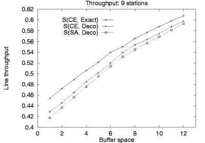
Figure 2:
Computed throughput of lines with OBA computed using
simulated annealing S(SA, Deco) compared with
complete enumerations using the exact S(CE, Exact) and
the decomposition evaluative methods S(CE, Deco).
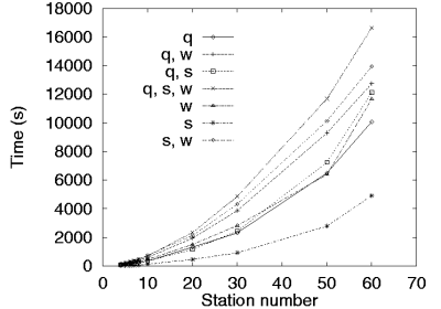
Figure 3:
Execution time for different measures of optimal configuration calculations
using the simulated annealing optimizer and the expansion method evaluator.


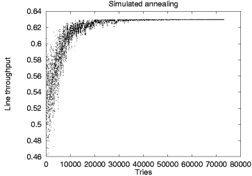
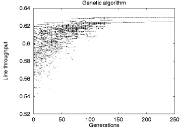
Figure 4:
Stochastic method operation comparison
We also used exPLOre in conjunction with algorithm animation techniques
[32] to visualize the search space of different
optimization algorithms in the temporal domain.
An interesting example of these results can be seen in Figure 4
where a graphical representation of the operation of the simulated annealing
optimizer appears beside the equivalent representation for the genetic
algorithm optimizer.
Each point on the two scatter charts represents a given line throughput value
at a specific step of the algorithm.
Both charts depict the calculation of the placement of 30 buffers in a balanced
line of 15 stations.
The simulated annealing algorithm optimizes a single solution in
the specific example in 80.000 iterations.
The solution's throughput value oscillates as both better and worse
solutions are randomly selected at each iteration step.
As can be seen on the chart, the oscillation width decreases following
the algorithm's exponential cooling schedule and converges towards the
optimal value.
In contrast to the simulated annealing algorithm, the genetic algorithm is
based on the implicit parallelism of the solutions represented by the
initial population.
Thus, in the specific example, it terminates with an optimal configuration
after 250 generations.
As the chart demonstrates, the search starts with a wide spectrum of
different solutions which are evaluated and evolve in parallel with
non-optimal solutions gradually becoming extinct.
Mutations and recombinations regenerate suboptimal solutions, but,
due to the probabilistic organism selection strategy, their survival
does not last for long.
5 Conclusions
ExPLOre was built from the bottom up as a workbench for experimenting
with production line optimization algorithms and methodologies.
It currently provides a rich set of algorithms for evaluating
production line configurations.
The architecture's modularity and the plug-compatibility of the
optimizer and throughput evaluator module instances have allowed us
to concentrate our work on an
objective comparison of the relative merits and deficiencies of the
various algorithms.
Placing methodologies which were up to now studied in isolation under
the same roof has provided us in some cases with surprisingly differing
results in terms of accuracy and efficiency for similar line configurations.
Thus part of our new work entails the reexamination and tuning of the
respective methods using exPLOre as an algorithm evaluation tool.
In addition, the modularity of exPLOre has prompted us to examine further
optimization and evaluation algorithms as candidates for inclusion.
We are currently working on fine-tuning the exPLOre optimizer based on
genetic algorithms.
Finally, a further direction of our research concerns the publication
of the exPLOre module port specifications and the provision of a friendly
user-interface in order to create a publicly available version as a standard
production line optimization algorithm workbench.
References
- [1]
-
H. T. Papadopoulos and C. Heavey.
Queueing Theory in Manufacturing Systems Analysis and Design: A
Classification of Models for Production and Transfer Lines.
European J. Oper. Res., 92:1-27, 1996.
- [2]
-
R. G. Askin and C. R. Standridge.
Modeling and Analysis of Manufacturing Systems.
John Wiley, New York, 1993.
- [3]
-
J. A. Buzacott and J. G. Shanthikumar.
Stochastic Models of Manufacturing Systems.
Prentice Hall, New Jersey, 1993.
- [4]
-
S. B. Gershwin.
Manufacturing Systems Engineering.
Prentice Hall, New Jersey, 1994.
- [5]
-
H. T. Papadopoulos, C. Heavey, and J. Browne.
Queueing Theory in Manufacturing Systems Analysis and Design.
Chapman and Hall, London, 1993.
- [6]
-
N. Viswanadham and Y. Narahari.
Performance Modeling of Automated Manufacturing Systems.
Prentice Hall, New Jersey, 1992.
- [7]
-
T. Altiok.
Performance Analysis of Manufacturing Systems.
Springer-Verlag, New York, 1997.
- [8]
-
D. Spinellis and C. T. Papadopoulos.
A Simulated Annealing Approach for Buffer Allocation in Reliable
Production Lines.
Annals of Operations Research, 93:373-384, 2000.
- [9]
-
J. Rumbaugh, I. Jacobson, and G. Booch.
The Unified Modeling Language Reference Manual.
Addison-Wesley, 1999.
- [10]
-
D. Spinellis and V. Guruprasad.
Lightweight Languages as Software Engineering Tools.
In J. C. Ramming, editor, USENIX Conference on Domain-Specific
Languages, pages 67-76, Santa Monica, CA, USA, Oct. 1997. Usenix
Association.
- [11]
-
V. Cerny.
Thermodynamical Approach to the Traveling Salesman Problem: an
Efficient Simulation Algorithm.
J. Optim. Theory Appl., 45:41-51, 1985.
- [12]
-
P. J. M. Van Laarhoven and E. H. L. Aarts.
Simulated Annealing: Theory and Applications.
D. Reidel, Dordrecht, The Nethelands, 1987.
- [13]
-
N. Metropolis, A. N. Rosenbluth, M. N. Rosenbluth, A. H. Teller, and E. Teller.
Equation of State Calculation by Fast Computing Machines.
J. Chem. Phys., 21(6):1087-1092, 1953.
- [14]
-
S. Kirkpatrick, C. D. G. Jr., and M. P. Vecchi.
Optimization by Simulated Annealing.
Science, 220:671-679, 1983.
- [15]
-
J. H. Holland.
Adaptation in Natural and Artificial Systems.
University of Michigan Press, Ann Arbor, Michigan, 1975.
- [16]
-
D. E. Goldberg.
Genetic Algorithms: In Search of Optimization & Machine
Learning.
Addison-Wesley, 1989.
- [17]
-
F. Glover.
Tabu Search - Part I.
ORSA Journal on Computing, 1:190-206, 1990.
- [18]
-
R. Gupta, S. A. Smolka, and S. Bhaskar.
On Randomization in Sequential and Distributed Algorithms.
ACM Comput. Surv., 26(1):7-86, 1994.
- [19]
-
A. Corana, M. Marchesi, C. Martini, and S. Ridella.
Minimizing Multimodal Functions of Continuous Variables with the
``Simulated Annealing'' Algorithm.
ACM Trans. Math. Software, 13(3):262-280, Sept. 1987.
- [20]
-
W. H. Press, B. P. Flannery, S. A. Teukolsky, and W. T. Vetterling.
Numerical Recipes in C, pages 343-352.
Cambridge University Press, 1988.
- [21]
-
R. W. Eglese.
Simulated Annealing: A Tool for Operational Research.
European J. Oper. Res., 46:271-281, 1990.
- [22]
-
C. Koulamas, S. R. Antony, and R. Jaen.
A Survey of Simulated Annealing Applications to Operations Research
Problems.
Omega International Journal of Management Science,
22(1):41-56, 1994.
- [23]
-
S. Forrest.
Genetic Algorithms.
ACM Comput. Surv., 28(1):77-83, Mar. 1996.
- [24]
-
C. L. Karr.
Genetic Algorithms for Modelling, Design, and Process Control.
In CIKM '93. Proceedings of the Second International
Conference on Information and Knowledge Management, pages 233-238. ACM,
1993.
- [25]
-
D. E. Goldberg.
Genetic and Evolutionary Algorithms Come of Age.
Commun. ACM, 37(3):113-119, Mar. 1994.
- [26]
-
G. Tompkins and F. Azadivar.
Genetic Algorithms in Optimizing Simulated Systems.
In WSC '95. Proceedings of the 1995 Conference on Winter
Simulation, pages 757-762. ACM, 1995.
- [27]
-
D. Spinellis and C. Papadopoulos.
Stochastic Algorithms for Buffer Allocation in Reliable Production
Lines.
Mathematical Problems in Engineering, 5:441-458, 2000.
- [28]
-
C. Heavey, H. T. Papadopoulos, and J. Browne.
The Throughput Rate of Multistation Unreliable Production Lines.
European J. Oper. Res., 68:69-89, 1993.
- [29]
-
S. B. Gershwin.
An Efficient Decomposition Method for the Approximate Evaluation of
Tandem Queues with Finite Storage Space and Blocking.
Oper. Res., 35(2):291-305, 1987.
- [30]
-
Y. Dallery and Y. Frein.
On Decomposition Methods for Tandem Queueing Networks with Blocking.
Oper. Res., 41(2):386-399, 1993.
- [31]
-
L. Kerbache and J. M. Smith.
The Generalized Expansion Method for Open Finite Queueing Networks.
European J. Oper. Res., 32:448-461, 1987.
- [32]
-
J. L. Bentley and B. W. Kernighan.
A System for Algorithm Animation.
Computing Systems, 4(1):5-30, Winter 1991.
Footnotes:
1
An earlier version of this paper appears in Dimitris K. Despotis and
Constantin Zopounidis, editors, Proceedings of the 5th International
Conference of the Decision Sciences Institute, DSI '99,
pages 1446-1449, Athens, Greece, July 1999. Decision Sciences Institute.
